import numpy as np
import pandas as pd
import matplotlib.pyplot as plt
import matplotlib as mpl
%matplotlib inline

import networkx as nxNetwork Science - UDD
Network metrics
Cristian Candia-Castro Vallejos, Ph.D.\(^{1,2}\)
Yessica Herrera-Guzmán, Ph.D.\(^{2, 3}\)
- [1] Data Science Institute (IDS), Universidad del Desarrollo,Chile
- [2] Northwestern Institute on Complex Systems, Kellogg School of Management, Northwestern Unviersity, USA
- [3] Center for Complex Network Research (CCNR), Northwestern Unviersity, USA
file_path = "edgelist.txt"g = nx.Graph()with open(file_path, "r") as file:
for line in file:
# Split each line to extract the node pairs
nodes = line.strip().split()
if len(nodes) == 2:
g.add_edge(nodes[0], nodes[1])# Fruchterman-Reingold force-directed layout algorithm ~ default
fig = plt.figure(figsize=(6,6))
nx.draw(g, node_size=40)
# if you need labels to check nodes:
# nx.draw(g, node_size=40, with_labels=True)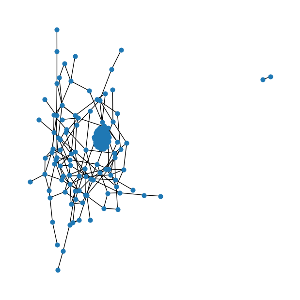
Three basic properties
N = len(g)
L = g.size()
degrees = list(dict(g.degree()).values())
kmin = min(degrees)
kmax = max(degrees)print("Number of nodes: ", N)
print("Number of links: ", L)
print('-------')
print("Average degree: ", 2*L/N) #Formula vista en clases (qué sucedía con las redes reales?)
print("Average degree (alternative estimation)", np.mean(degrees))
print('-------')
print("Minimum degree: ", kmin)
print("Maximum degree: ", kmax)Number of nodes: 197
Number of links: 1651
-------
Average degree: 16.761421319796955
Average degree (alternative estimation) 16.761421319796955
-------
Minimum degree: 1
Maximum degree: 43Degree distribution
bin_edges = np.logspace(np.log10(kmin), np.log10(kmax), num=20)

# remember to make the histogram!
density, _ = np.histogram(degrees, bins=bin_edges, density=True)
fig = plt.figure(figsize=(4,4))
log_be = np.log10(bin_edges) # log scale
x = 10**((log_be[1:] + log_be[:-1])/2) # (X_i+X_(i+1))/2
plt.loglog(x, density, marker='o', linestyle='none')
# don't forget axis labels and right size!
plt.xlabel(r"degree $k$", fontsize=16)
plt.ylabel(r"$P(k)$", fontsize=16)
plt.show()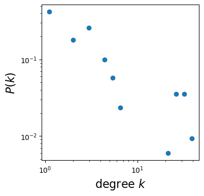
# Check binning
fig = plt.figure(figsize=(4,4))

a=bin_edges[1:] - bin_edges[:-1]

plt.plot(a, color='blue', lw=2)

plt.show()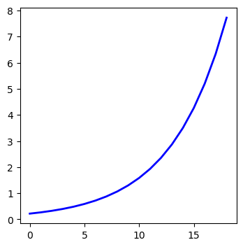
Path length
nx.average_shortest_path_length(g)--------------------------------------------------------------------------- NetworkXError Traceback (most recent call last) Input In [117], in <cell line: 1>() ----> 1 nx.average_shortest_path_length(g) File ~/miniconda3/envs/otro_lumos/lib/python3.8/site-packages/networkx/algorithms/shortest_paths/generic.py:389, in average_shortest_path_length(G, weight, method) 387 raise nx.NetworkXError("Graph is not weakly connected.") 388 if not G.is_directed() and not nx.is_connected(G): --> 389 raise nx.NetworkXError("Graph is not connected.") 391 # Compute all-pairs shortest paths. 392 def path_length(v): NetworkXError: Graph is not connected.
Oh! Grapht is not connected!
How do we measure the average path length, then?
# Explore number of connected components
components = list(nx.connected_components(g))
largest_component = max(components, key=len)# This is a subgraph of the largest connected component
lc_graph = g.subgraph(largest_component)nx.average_shortest_path_length(lc_graph)1.696969696969697nx.diameter(lc_graph)2Quick quizz:
How are the average shorthest path and diameter related?
What do they measure drom the network structure?
How would the diameter change for a random network of N nodes, when changed to a tree-like structure?
Compute the size of the largest connected component: number of nodes and edges respect to the entire network.
Clustering coefficient
clustering = nx.clustering(g)clustering_values = list(clustering.values())plt.hist(clustering_values, bins=20, alpha=0.7)
plt.xlabel("Clustering Coefficient")
plt.ylabel("Frequency")
plt.title("Clustering Coefficient Distribution")
plt.grid(True)
# Show the histogram
plt.show()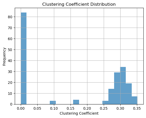
Note that nx.clustering(g) provides the clustering for each node. So you can explore what is the clustering coefficient of specific nodes, for example:
node_id = '87'
cc_node = nx.clustering(g, node_id)
print(f"Clustering coefficient for Node {node_id}: {cc_node}")
Clustering coefficient for Node 87: 0.16666666666666666Now we know the distribution of the clustering coefficient, let’s compute the average clustering coefficient:
average_cc = nx.average_clustering(g)
print(f"The average clustering coefficient of this network is {average_cc}")
The average clustering coefficient of this network is 0.1682917533972737Lastly, let’s compute network density:
density = nx.density(g)
print(f"The density of this network is {density}")
The density of this network is 0.08551745571324977Quick quizz:
What is the meaning of a high clustering coefficient?
What is the meaning of a low clustering coefficient?
How is the density of a network related to clustering coefficient?
How does the average clustering coefficient varies by each network model: random, BA, and WS?
What insights could you obtain about a network by only knowing that its average clustering coefficient is 0.46 and it has a 30% of random edges?
Lastly, describe what is the usefulness of the three network metrics for network analysis.
Network properties of different networks
Erdos-Renyi random graph
num_nodes = 200# Probability of edge creation (adjust and have fun learning!)
probability = 0.2er = nx.erdos_renyi_graph(num_nodes, probability)fig = plt.figure(figsize=(6,6))
nx.draw(er, node_size=40)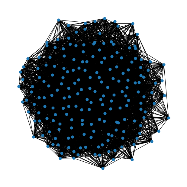
Watts-Strogatz small-world graph
num_nodes = 200# Number of nearest neighbors to connect
k = 4# Probability of rewiring each edge
p = 0.1ws = nx.watts_strogatz_graph(num_nodes, k, p)fig = plt.figure(figsize=(6,6))
nx.draw(ws, node_size=40)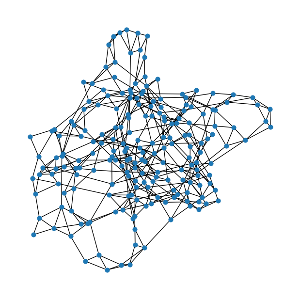
Barabási-Albert graph
num_nodes = 200# Number of edges to attach from a new node to existing nodes ~ Hubs!
m = 3ab = nx.barabasi_albert_graph(num_nodes, m)fig = plt.figure(figsize=(6,6))
nx.draw(ab, node_size=40)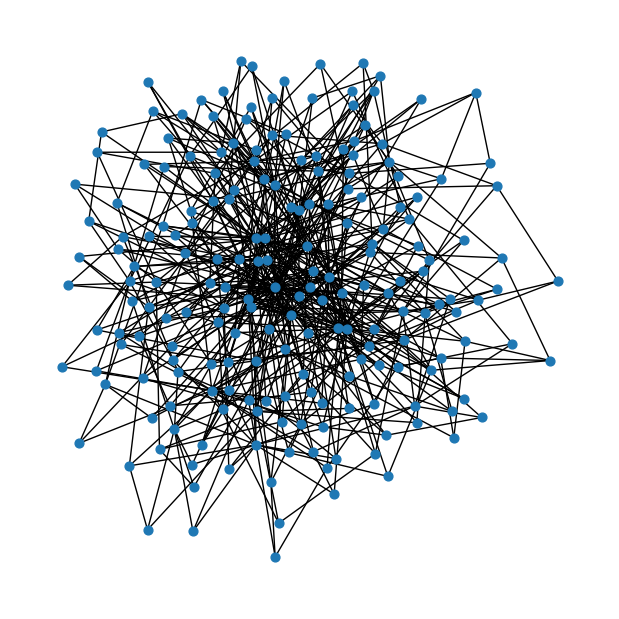
Moving on:
Compute the network properties studied here for each of these networks.
Describe whether the three central metrics can be characteristic of each model.
Discuss the limitations of the metrics and what other metrics could be computed to understand the network and nodes’ relationships in more detail.